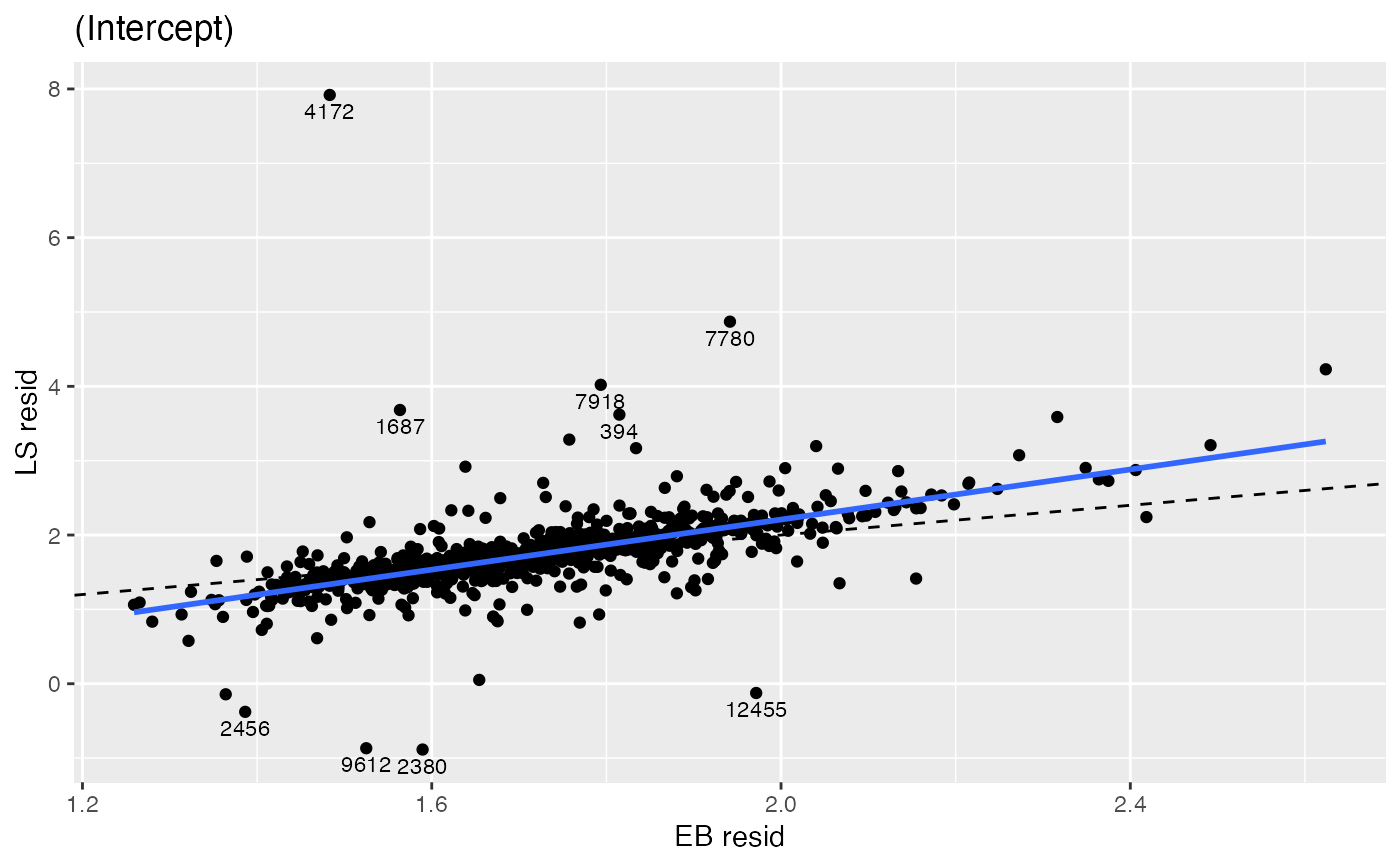
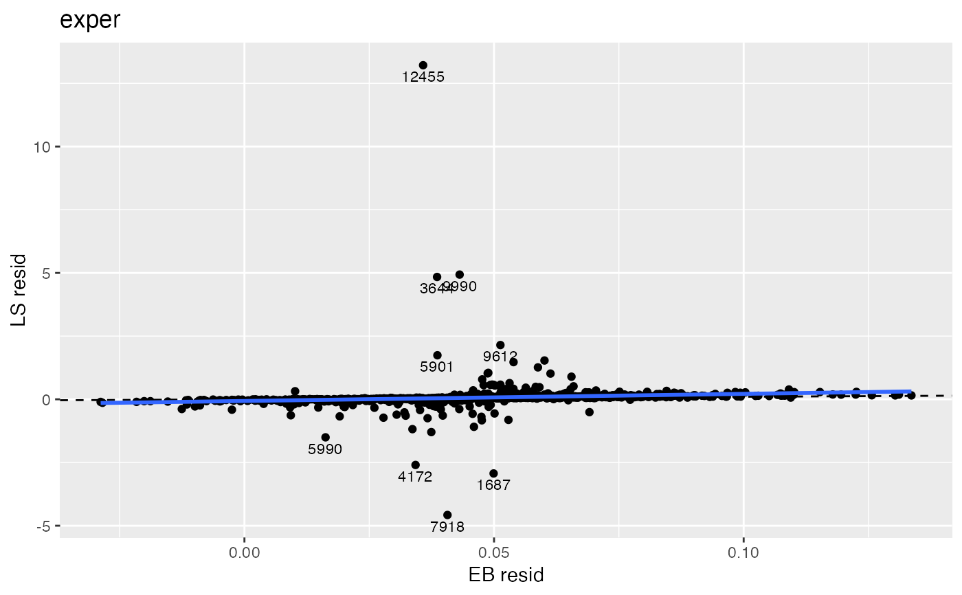
Visually comparing shrinkage and LS estimates
Source:R/group_level_residual_functions.R
compare_eb_ls.RdThis function creates a plot (using qplot()) where the shrinkage
estimate appears on the horizontal axis and the LS estimate appears on the
vertical axis.
compare_eb_ls(eb, ols, identify = FALSE, silent = TRUE, ...)
Arguments
| eb | a matrix of random effects |
|---|---|
| ols | a matrix of the OLS estimates found using |
| identify | the percentage of points to identify as unusual,
|
| silent | logical: should the list of data frames used to make the plots be suppressed. |
| ... | other arguments to be passed to |
Author
Adam Loy loyad01@gmail.com
Examples
#> Warning: Model failed to converge with max|grad| = 0.00609024 (tol = 0.002, component 1)wages.sepLM <- adjust_lmList(lnw ~ exper | id, data = wages) rancoef.eb <- coef(wages.fm1)$id rancoef.ols <- coef(wages.sepLM) compare_eb_ls(eb = rancoef.eb, ols = rancoef.ols, identify = 0.01)#>#>#> Warning: Removed 38 rows containing non-finite values (stat_smooth).#> Warning: Removed 38 rows containing missing values (geom_point).

