Quantile-quantile confidence bands

Draws quantile-quantile confidence bands, with an additional detrend option.

geom_qq_band(
  mapping = NULL,
  data = NULL,
  stat = "qq_band",
  position = "identity",
  na.rm = TRUE,
  show.legend = NA,
  inherit.aes = TRUE,
  distribution = "norm",
  dparams = list(),
  detrend = FALSE,
  identity = FALSE,
  qtype = 7,
  qprobs = c(0.25, 0.75),
  bandType = "pointwise",
  B = 1000,
  conf = 0.95,
  mu = NULL,
  sigma = NULL,
  ...
)

stat_qq_band(
  mapping = NULL,
  data = NULL,
  geom = "qq_band",
  position = "identity",
  na.rm = TRUE,
  show.legend = NA,
  inherit.aes = TRUE,
  distribution = "norm",
  dparams = list(),
  detrend = FALSE,
  identity = FALSE,
  qtype = 7,
  qprobs = c(0.25, 0.75),
  bandType = "pointwise",
  B = 1000,
  conf = 0.95,
  mu = NULL,
  sigma = NULL,
  ...
)

Arguments

mapping	Set of aesthetic mappings created by aes() or aes_(). If specified and inherit.aes = TRUE (the default), it is combined with the default mapping at the top level of the plot. You must supply mapping if there is no plot mapping.
data	The data to be displayed in this layer. There are three options: If NULL, the default, the data is inherited from the plot data as specified in the call to ggplot(). A data.frame, or other object, will override the plot data. All objects will be fortified to produce a data frame. See fortify() for which variables will be created. A function will be called with a single argument, the plot data. The return value must be a data.frame, and will be used as the layer data. A function can be created from a formula (e.g. ~ head(.x, 10)).
stat	statistic to use to calculate confidence bands. Should be `qq_band`.
position	Position adjustment, either as a string, or the result of a call to a position adjustment function.
na.rm	If FALSE, the default, missing values are removed with a warning. If TRUE, missing values are silently removed.
show.legend	logical. Should this layer be included in the legends? NA, the default, includes if any aesthetics are mapped. FALSE never includes, and TRUE always includes. It can also be a named logical vector to finely select the aesthetics to display.
inherit.aes	If FALSE, overrides the default aesthetics, rather than combining with them. This is most useful for helper functions that define both data and aesthetics and shouldn't inherit behaviour from the default plot specification, e.g. borders().
distribution	Character. Theoretical probability distribution function to use. Do not provide the full distribution function name (e.g., "dnorm"). Instead, just provide its shortened name (e.g., "norm"). If you wish to provide a custom distribution, you may do so by first creating the density, quantile, and random functions following the standard nomenclature from the stats package (i.e., for "custom", create the dcustom, pcustom, qcustom, and rcustom functions).
dparams	List of additional parameters passed on to the previously chosen distribution function. If an empty list is provided (default) then the distributional parameters are estimated via MLE. MLE for custom distributions is currently not supported, so you must provide the appropriate dparams in that case.
detrend	Logical. Should the plot objects be detrended? If TRUE, the objects will be detrended according to the reference Q-Q line. This procedure was described by Thode (2002), and may help reducing visual bias caused by the orthogonal distances from Q-Q points to the reference line.
identity	Logical. Should an identity line be used as the reference line used to construct the confidence bands? If TRUE, the identity line is used. If FALSE (default), the commonly-used Q-Q line that intercepts two data quantiles specified in qprobs is used. Please notice that the chosen reference line will also be used for the detrending procedure, if detrend = TRUE.
qtype	Integer between 1 and 9. Type of the quantile algorithm to be used by the quantile function to construct the Q-Q line.
qprobs	Numeric vector of length two. Represents the quantiles used by the quantile function to construct the Q-Q line.
bandType	Character. Either "pointwise", "boot", "ks" or "ts". "pointwise" constructs pointwise confidence bands based on Normal confidence intervals. "boot" creates pointwise confidence bands based on a parametric bootstrap; parameters are estimated with MLEs. "ks" constructs simultaneous confidence bands based on the Kolmogorov-Smirnov test. Finally, "ts" constructs tail-sensitive confidence bands, as described by Aldor-Noiman et al. (2013) (also, see 'Note' for limitations).
B	Integer. If bandType = "boot", then B is the number of bootstrap replicates. If bandType = "ts", then B is the number of simulated samples.
conf	Numerical. Confidence level of the bands.
mu	Numerical. Only used if bandType = "ts". Center distributional parameter used to construct the simulated tail-sensitive confidence bands. If either mu or sigma are NULL, then those parameters are estimated using Qn and s_Qn, respectively.
sigma	Numerical. Only used if bandType = "ts". Scale distributional parameter used to construct the simulated tail-sensitive confidence bands. If either mu or sigma are NULL, then those parameters are estimated using robust estimates from the stats package.
...	Other arguments passed on to layer(). These are often aesthetics, used to set an aesthetic to a fixed value, like colour = "red" or size = 3. They may also be parameters to the paired geom/stat.
geom	The geometric object to use display the data

Note

• Tail-sensitive confidence bands are only implemented for Normal Q-Q plots. As a future update, we intend to generalize to other distributions.

• Bootstrap bands are constructed based on a MLE parametric bootstrap. Hence, it is not possible to construct such bands if the sample and theoretical distributions present mismatching supports.

References

• Thode, H. (2002), Testing for Normality. CRC Press, 1st Ed.

• Aldor-Noiman, S. et al. (2013). The Power to See: A New Graphical Test of Normality. The American Statistician. 67:4.

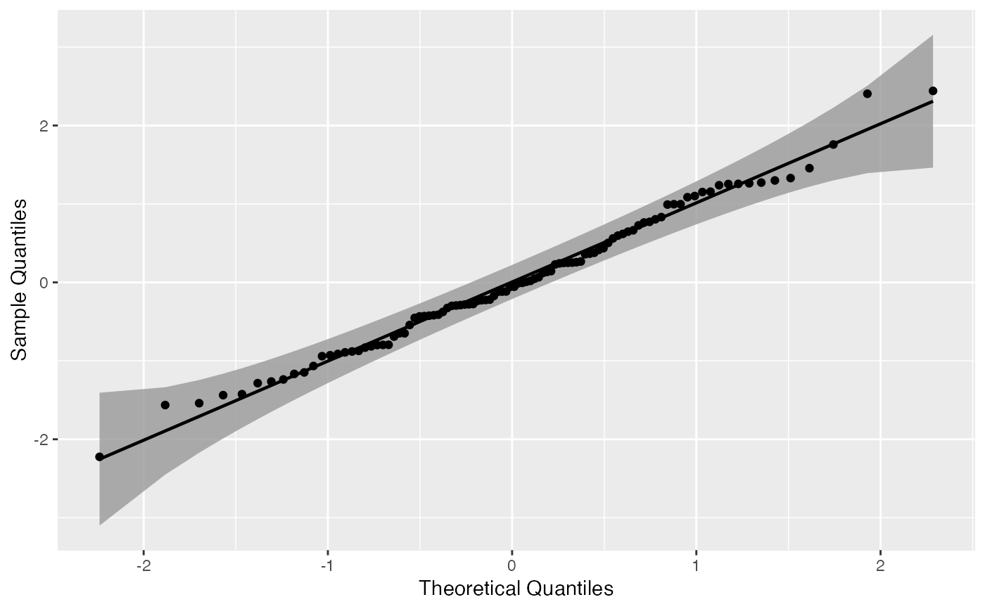
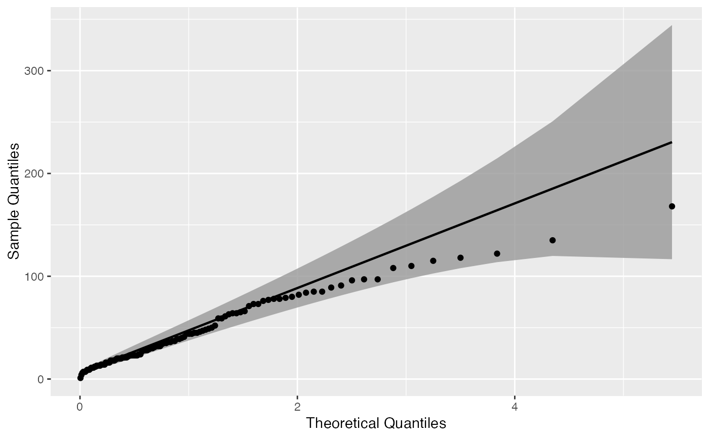
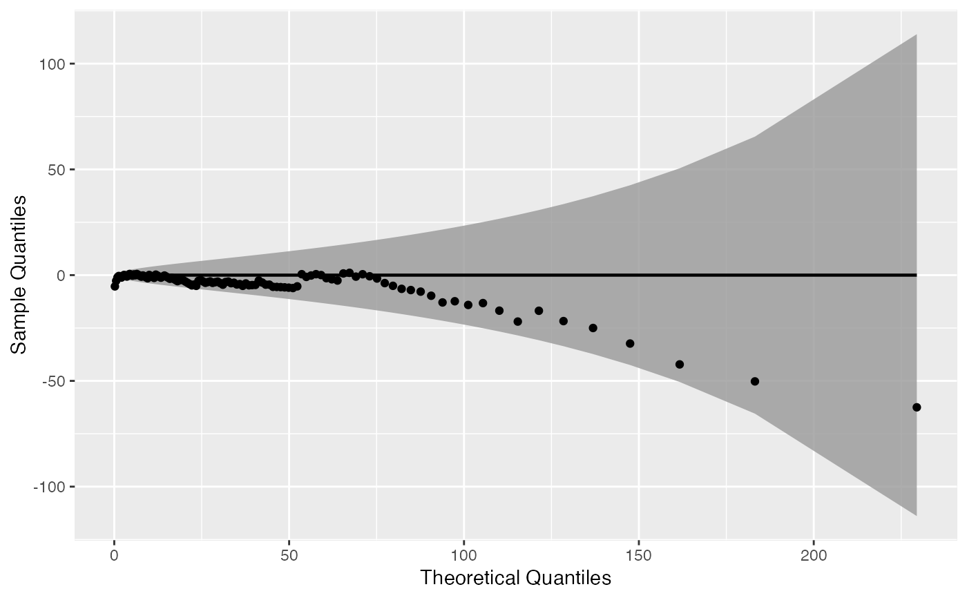
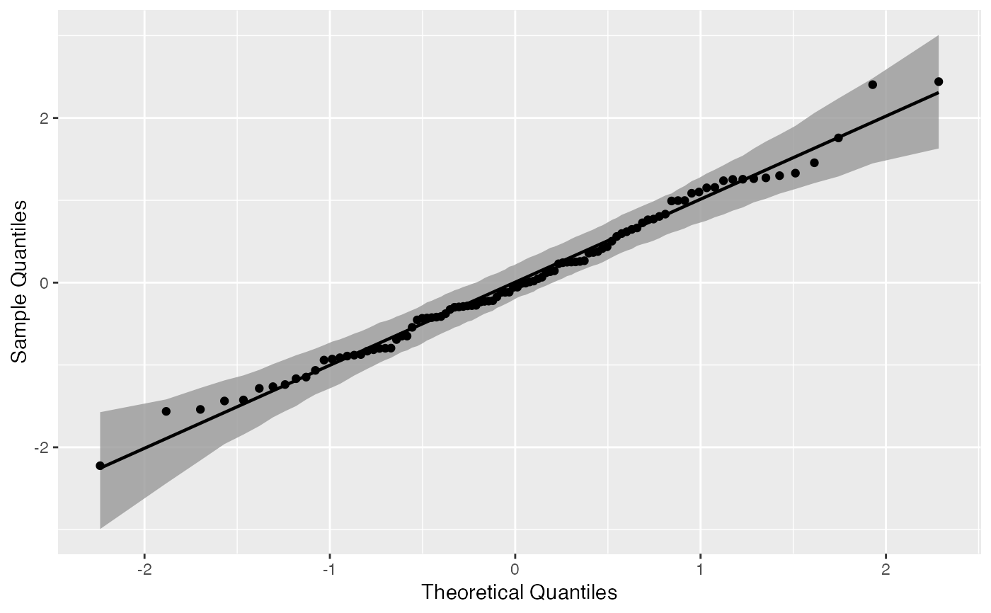
Examples

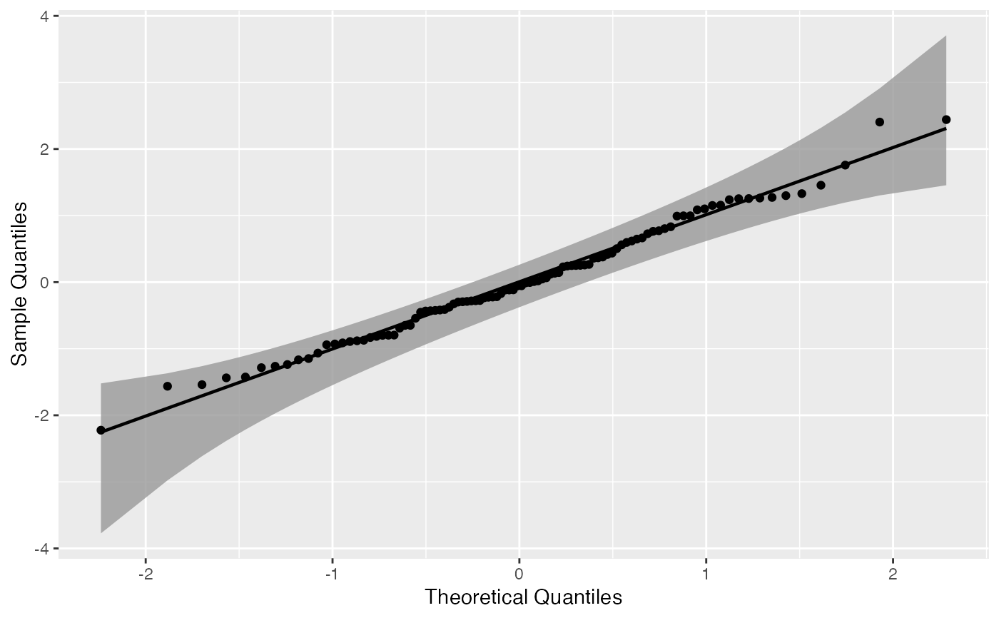
# generate random Normal data
set.seed(0)
smp <- data.frame(norm = rnorm(100))

# Normal Q-Q plot of Normal data
gg <- ggplot(data = smp, mapping = aes(sample = norm)) +
 stat_qq_band() +
 stat_qq_line() +
 stat_qq_point()
gg + labs(x = "Theoretical Quantiles", y = "Sample Quantiles")

# Exponential Q-Q plot of mean ozone levels (airquality dataset)
di <- "exp"
dp <- list(rate = 1)
gg <- ggplot(data = airquality, mapping = aes(sample = Ozone)) +
 stat_qq_band(distribution = di, dparams = dp) +
 stat_qq_line(distribution = di, dparams = dp) +
 stat_qq_point(distribution = di, dparams = dp) +
 labs(x = "Theoretical Quantiles", y = "Sample Quantiles")
gg

# Detrended Exponential Q-Q plot of mean ozone levels
di <- "exp"
dp <- list(rate = 1)
de <- TRUE
gg <- ggplot(data = airquality, mapping = aes(sample = Ozone)) +
 stat_qq_band(distribution = di, detrend = de) +
 stat_qq_line(distribution = di, detrend = de) +
 stat_qq_point(distribution = di, detrend = de) +
 labs(x = "Theoretical Quantiles", y = "Sample Quantiles")
gg

# Normal Q-Q plot of Normal data with boostrap confidence bands
bt <- "boot"
gg <- ggplot(data = smp, mapping = aes(sample = norm)) +
 stat_qq_band(bandType = bt) +
 stat_qq_line() +
 stat_qq_point() +
 labs(x = "Theoretical Quantiles", y = "Sample Quantiles")
gg

# Normal Q-Q plot of Normal data with tail-sensitive confidence bands
bt <- "ts"
gg <- ggplot(data = smp, mapping = aes(sample = norm)) +
 stat_qq_band(bandType = bt) +
 stat_qq_line() +
 stat_qq_point() +
 labs(x = "Theoretical Quantiles", y = "Sample Quantiles")
gg