Probability-probability confidence bands — stat_pp

Draws probability-probability confidence bands.

stat_pp_band(
  mapping = NULL,
  data = NULL,
  geom = "ribbon",
  position = "identity",
  na.rm = TRUE,
  show.legend = NA,
  inherit.aes = TRUE,
  distribution = "norm",
  dparams = list(),
  bandType = "boot",
  B = 1000,
  conf = 0.95,
  detrend = FALSE,
  ...
)

Arguments

mapping	Set of aesthetic mappings created by `aes()` or `aes_()`. If specified and `inherit.aes = TRUE` (the default), it is combined with the default mapping at the top level of the plot. You must supply `mapping` if there is no plot mapping.
data	The data to be displayed in this layer. There are three options: If `NULL`, the default, the data is inherited from the plot data as specified in the call to `ggplot()`. A `data.frame`, or other object, will override the plot data. All objects will be fortified to produce a data frame. See `fortify()` for which variables will be created. A `function` will be called with a single argument, the plot data. The return value must be a `data.frame`, and will be used as the layer data. A `function` can be created from a `formula` (e.g. `~ head(.x, 10)`).
geom	The geometric object to use display the data
position	Position adjustment, either as a string, or the result of a call to a position adjustment function.
na.rm	If `FALSE`, the default, missing values are removed with a warning. If `TRUE`, missing values are silently removed.
show.legend	logical. Should this layer be included in the legends? `NA`, the default, includes if any aesthetics are mapped. `FALSE` never includes, and `TRUE` always includes. It can also be a named logical vector to finely select the aesthetics to display.
inherit.aes	If `FALSE`, overrides the default aesthetics, rather than combining with them. This is most useful for helper functions that define both data and aesthetics and shouldn't inherit behaviour from the default plot specification, e.g. `borders()`.
distribution	Character. Theoretical probability distribution function to use. Do not provide the full distribution function name (e.g., `"dnorm"`). Instead, just provide its shortened name (e.g., `"norm"`). If you wish to provide a custom distribution, you may do so by first creating the density, quantile, and random functions following the standard nomenclature from the `stats` package (i.e., for `"custom"`, create the `dcustom`, `pcustom`, `qcustom`, and `rcustom` functions).
dparams	List of additional parameters passed on to the previously chosen `distribution` function. If an empty list is provided (default) then the distributional parameters are estimated via MLE. MLE for custom distributions is currently not supported, so you must provide the appropriate `dparams` in that case.
bandType	Character. Only `"boot"` is available for now. `"boot"` creates pointwise confidence bands based on a bootstrap.
B	Integer. If `bandType = "boot"`, then `B` is the number of bootstrap replicates.
conf	Numerical. Confidence level of the bands.
detrend	Logical. Should the plot objects be detrended? If `TRUE`, the objects will be detrended according to the default identity P-P line. This procedure was described by Thode (2002), and may help reducing visual bias caused by the orthogonal distances from P-P points to the reference line.
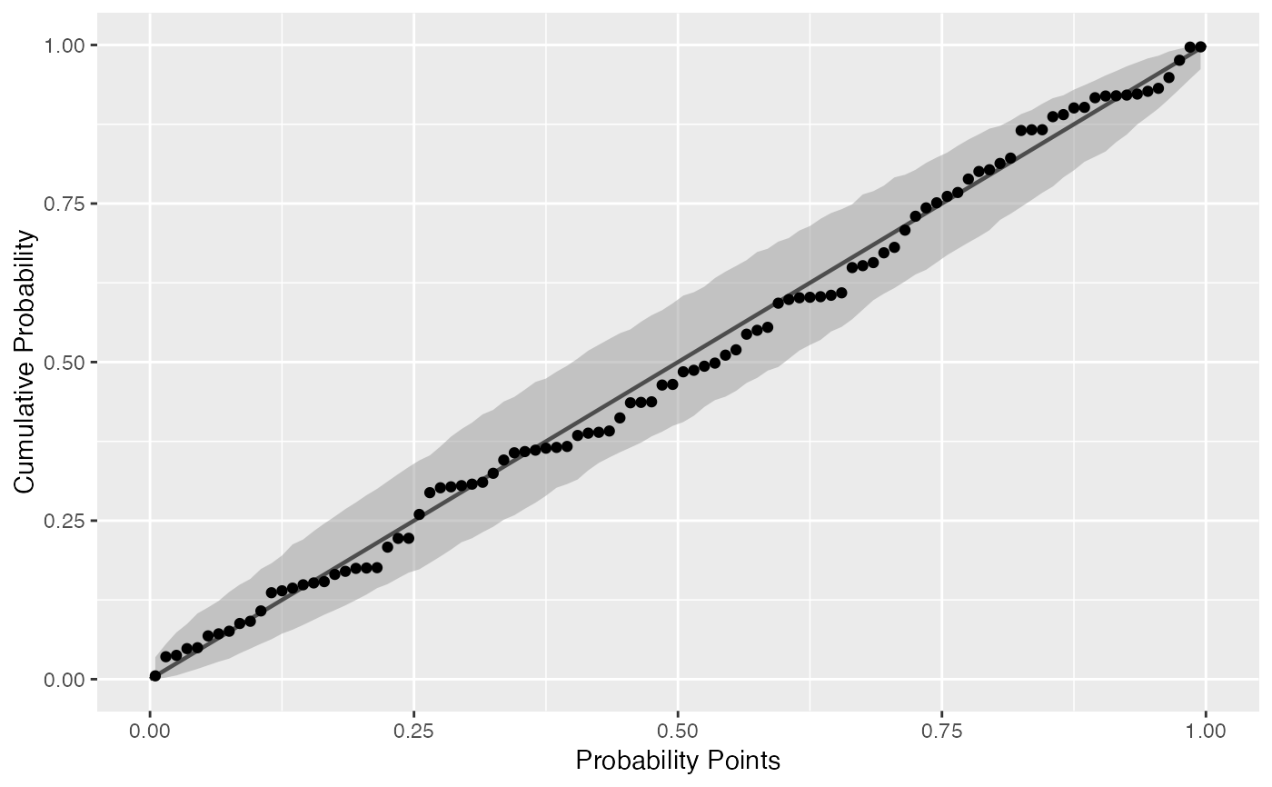
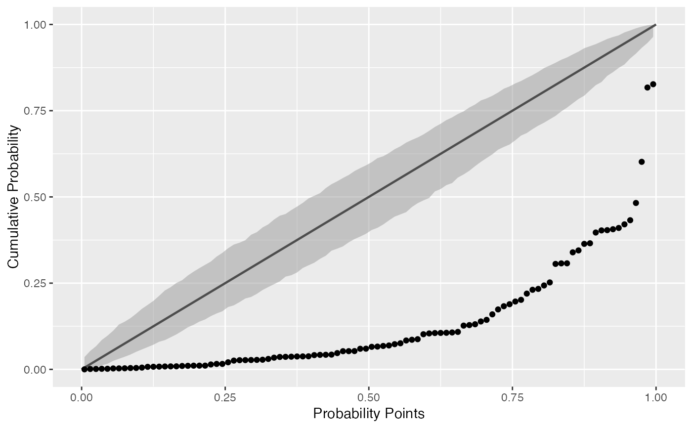
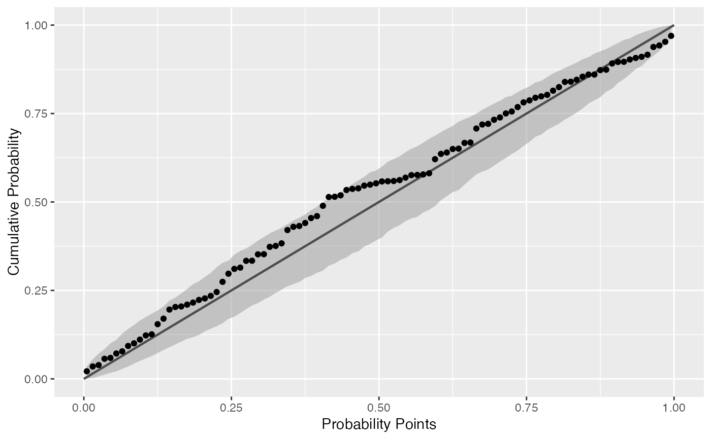
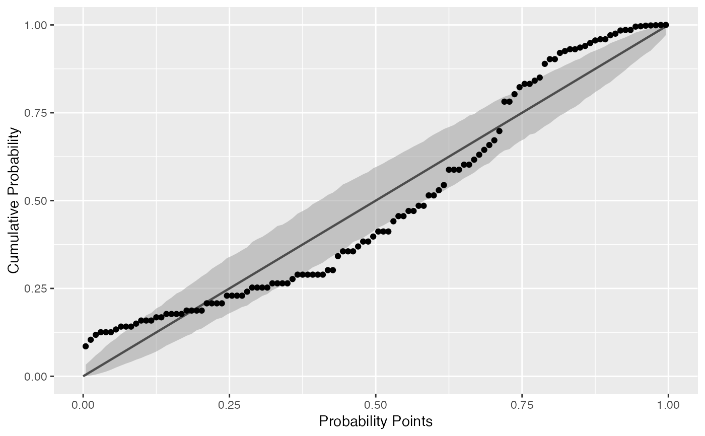
...	Other arguments passed on to `layer()`. These are often aesthetics, used to set an aesthetic to a fixed value, like `colour = "red"` or `size = 3`. They may also be parameters to the paired geom/stat.

Examples

# generate random Normal data
set.seed(0)
smp <- data.frame(norm = rnorm(100), exp = rexp(100))

# Normal P-P plot of Normal data
gg <- ggplot(data = smp, mapping = aes(sample = norm)) +
 stat_pp_band() +
 stat_pp_line() +
 stat_pp_point() +
 labs(x = "Probability Points", y = "Cumulative Probability")
gg

# Shifted Normal P-P plot of Normal data
dp <- list(mean = 1.5)
gg <- ggplot(data = smp, mapping = aes(sample = norm)) +
 stat_pp_band(dparams = dp) +
 stat_pp_line() +
 stat_pp_point(dparams = dp) +
 labs(x = "Probability Points", y = "Cumulative Probability")
gg

# Exponential P-P plot of Exponential data
di <- "exp"
gg <- ggplot(data = smp, mapping = aes(sample = exp)) +
 stat_pp_band(distribution = di) +
 stat_pp_line() +
 stat_pp_point(distribution = di) +
 labs(x = "Probability Points", y = "Cumulative Probability")
gg

# Normal P-P plot of mean ozone levels (airquality dataset)
dp <- list(mean = 38, sd = 27)
gg <- ggplot(data = airquality, mapping = aes(sample = Ozone)) +
 stat_pp_band(dparams = dp) +
 stat_pp_line() +
  stat_pp_point(dparams = dp) +
 labs(x = "Probability Points", y = "Cumulative Probability")
gg